Excel Vlookup Function Can Be Fun For Everyone

variety _ lookup: It is defined whether you want a specific or an approximate match. The feasible value is REAL or FALSE. Real value returns an approximate suit, and the INCORRECT value returns a precise suit. The IFERROR feature returns a value one specifies id a formula evaluates to an error, otherwise, returns the formula.

IFERROR look for the list below errors: #N/ A, #VALUE!, #REF!, #DIV/ 0!, #NUM!, #NAME?, or #NULL! Note: If lookup _ worth to be searched takes place greater than as soon as, then the VLOOKUP function will certainly locate the initial event of lookup _ worth. Below is the IFERROR Formula in Excel: The arguments of IFERROR function are clarified below: value: It is the value, referral, or formula to examine for an error.

While making use of the VLOOKUP function in MS Excel, if the value looked for is not found in the given data, it returns #N/ An error. Below is the IFERROR with VLOOKUP Solution in Excel: =IFERROR( VLOOKUP (lookup _ worth, table _ array, col _ index _ num, [variety _ lookup], worth _ if _ error) IFERROR with VLOOKUP in Excel is really easy as well as very easy to use.

You can download this IFERROR with VLOOKUP Excel Design Template right here-- IFERROR with VLOOKUP Excel Template Allow us take an instance of the basic pay of the employees of a firm. In the above number, we have a listing of worker ID, Worker Call as well as Staff member standard pay. Currently, we wish to browse the employees 'fundamental pay relative to the Employee ID 5902. In this scenario, VLOOKUP function will certainly return #N/ An error. So it is much better to replace the #N/ An error with a tailored value that every person can understand why the mistake is coming. So, we will use IFERROR with VLOOKUP Function in Excel in the list below means:=IFERROR (VLOOKUP (F 5, B 3:D 13, 3,0)," Information Not Discovered" )We will observe that the mistake has actually been replaced with the personalized worth "Information Not Found". We can utilize the function in the same workbook or from different workbooks by the use 3D

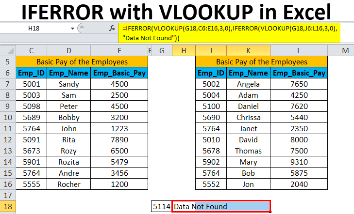
cell referencing. Let us take the example on the exact same worksheet to understand the use of the function on the fragmented datasets in the exact same worksheet. In the above figure, we have 2 collections of information of basic pay of the staff members. Currently, we wish to browse the employees' standard pay relative to the Staff member ID

All about How To Do A Vlookup

5902. We will utilize the adhering to formula for searching information in table 1:=VLOOKUP (G 18, C 6: E 16, 3, 0)The outcome will come as #N/ A. As the data browsed for is unavailable in the table 1 data collection. The staff member ID 5902 is offered in Table 2 information established. Currently, we want to compare both of the information sets

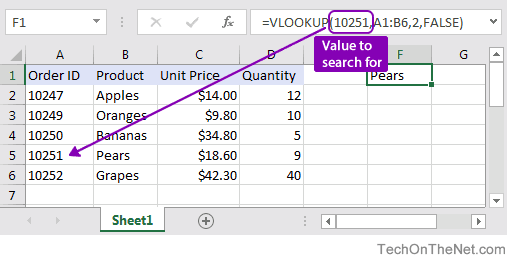
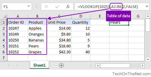
of table 1 as well as table 2 in a solitary cell as well as obtain the outcome. It is better to replace the #N/ An error with a personalized worth that everyone can understand why the mistake is coming. So, we will make use of IFERROR with VLOOKUP Function in Excel in the following way:=IFERROR(VLOOKUP(lookup _ worth, table _ selection, col _ index _ num, [variety _ lookup], IFERROR (VLOOKUP (lookup _ value, table _ selection, col _ index _ num, [variety _ lookup], worth _ if _ error)) We have utilized the feature in the instance in the following method: =IFERROR(VLOOKUP(G 18, C 6: E 16, 3,0), IFERROR (VLOOKUP (G 18, J 6: L 16, 3, 0),"Information Not Discovered"))As the employee ID 5902 is offered in the table 2 information established, the outcome will reveal as 9310. Pros: Helpful to trap and also manage mistakes generated by various other formulas or features. IFERROR look for the list below mistakes: #N/ A, #VALUE!, #REF!, #DIV/ 0!, #NUM!, #NAME?, or #NULL! Disadvantages: IFERROR changes all kinds of mistakes with the customized worth. If any kind of other errors except the #N/ A happen, still the tailored value specified will be checked out in the outcome. If value _ if _ error is offered as a vacant message(""), nothing is presented also when a mistake is found. If IFERROR is given as a table selection formula, it returns an array of outcomes with one product per cell in the value area. This has been a guide to IFERROR with VLOOKUP in Excel. You can also gowith our various other recommended short articles-- Exactly how to Utilize RANKING Excel Feature Feature HLOOKUP Feature in Excel With Examples Exactly How To Use ISERROR Function in Excel. VLOOKUP is an exceptionally beneficial formula in Excel. Sadly -- for the SEM newbie-- it is likewise among the most complex when you are simply starting out. Given that I 'm a relative newbie in paid search, the force of my work is production tasks. VLOOKUP is something that I make use of every single day. Naturally I asked for aid, but learning VLOOKUP from someone that already recognized it as well as its details proved to be not so practical. I desperately desired somebody to just lay it out in the simplest, most stripped-down way possible. To make sure that's what I will do for you right here: I'll walk you through the framework actions that I want I had actually understood. I don't even understand everything it can do yet. )According to Excel's formula description, VLOOKUP"seeks a value in the leftmost column of a table, and after that returns a value in the very same row from a column you specify. "Super useful, right? To stupid it down for you

, VLOOKUP allows you pull information about your selected cells into your present sheet, from other sheets or workbooks where that worth exists. CPC for each key words is. You have an additional sheet that is a keyword report with all the data for every single key words in the account-- this will be called Search phrase Sheet. You can stay clear of by hand sorting through every one of those keyword phrases and needing to duplicate and also paste the Avg. CPCs by utilizing VLOOKUP.

excel vlookup help vlookup in excel isna excel vlookup unsorted list